STaR-Bets: Sequential Target-Recalculating Bets for Tighter Confidence Intervals
This work was done in collaboration with Francesco Orabona
Intro
Confidence intervals are fundamental tools not only in statistics, but in virtually every field of science where we quantify statistical significance. We have a good understanding of the asymptotical width of the confidence intervals – it should be $\sqrt{2\sigma^2\log\frac1 \delta/n}$ as predicted the central limit theorem – but for small sample sizes (think of $< 1000$), we do not know much. The classical concentration inequalities of Hoeffding and Bernstein (and the Maurer and Pontil variant) have the correct leading constants, but empirically they do not work well in the small sample regime. In this blogpost, I walk you through our paper where we construct short confidence intervals performing well for all sample sizes.
Technicalities
We consider an $i.i.d.$ sample of $n$ realizations of a random variable $X$ supported on $[0,1]$ with mean $\mu$ and variance $\sigma^2$, and construct a $1-\delta$ lower confidence bound $\text{LCB}_\delta$; that is, $\mathbb{P}(\mu \geq \text{LCB}_\delta(X_1, \dots, X_n)) \geq 1-\delta$.
The Betting Framework for Hypothesis Testing
We adopt the testing-by-betting framework. For illustration, suppose you want to test whether a coin is fair, we make it the null hypothesis: $H_0: \mathbb{P}(\text{heads} = 0.5)$. Next, we set up a betting game where you sequentially bet on the outcomes of the coin and either win or lose the staked amount. For example, start with initial wealth of $W_0 = 1$. Bet $0.2$ on heads and observe heads, now you have wealth $W_1 = 1.2$ etc. If the game is fair, it is unlikely that you make money. But if you do make substantial money, that’s evidence the coin isn’t fair!
More generally - under the null hypothesis - the sequences of wealth values $W_0, W_1, \ldots, W_n$ is a suprmartingale; that is, it satisfies: \(\mathbb{E}[W_{i+1} \mid W_0, \ldots, W_i] \leq W_i,\) implying that we are not making money in expectation. We also require $W_i \geq 0$; that is, one cannot borrow money. By Markov’s inequality, as soon as $W_n \geq \frac{W_0}{\delta}$, we reject the null hypothesis at confidence level $1-\delta$. For simplicity, we adopt a convention that $W_0 =1$.
Confidence Intervals by Betting
We have just described how to test a hypothesis that the coin is fair. We can simply extend the procedure to test if $\mu = m$ by constructing a betting game that is fair if $\mu = m$ holds true. We perform the test for all values of $m \in [0,1]$ and the confidence set is the set for which we did not win enough money in the betting game. It looks suspicious that I have just told you to play an infinite (even uncountable) number of betting games, but it is not a problem and we can play them implicitly. For instance, we (actually) play them for $m \in \{0, t, 2t, \dots, 1-t, 1\}$ and we can show that in the game testing $\mu = m = k+t$, we make more money than when testing $\mu = m’ = k+\tau$ for $\tau \in [0,t]$, and so we play the continuum of betting games only implicitly.
Hoeffding Betting: A Simple Example
We derive Hoeffding’s inequality in this framework. The game is constructed by Hoeffding’s lemma:
\begin{align} M(\ell) = e^{\ell (X-\mu) - \ell^2/8} && \mathbb{E}[M(\ell)]\leq 1. \end{align} That is, we select $\ell$, and then, after observing $X$, we multiply our wealth by $M(\ell)$. It holds that $\mathbb{E}[W_{i+1} | W_0, \dots, W_i] = \mathbb{E}\left[ W_iM(\ell) \right] \leq W_i$ and $W_i \geq 0$ as $W_0=1$; thus, it is a supermartingale. Simple calculations show that the optimal constant bet resulting in the shortest confidence interval is
\[\ell_H = \sqrt{\frac{8\log\frac{1}{\delta}}{n}},\]recovering Hoeffding’s inequality after straightforward algebraic manipulations. However, there is no reason for choosing a betting strategy beforehand and sticking to it as we will see now.
STaR: Sequential Target-Recalculating Bets
Our key insight is that optimal betting should adapt based on the current situation. We call algorithms that do this STaR algorithms (Sequential Target-Recalculating). Conceptually speaking, we do not want to bet based on what was the game initially, but rather on how is the game now. A STaR algorithm uses two pieces of information at each step $t$:
- $\log\frac{1}{W_t \delta}$ - how much times we still need to multiply our wealth (instead of $\log\frac1\delta$).
- $n - t + 1$ - how many rounds remain (instead of $n$).
Thus, STaR-Hoeffding at time $t$ uses the bet that is the optimal constant bet for the remaining rounds:
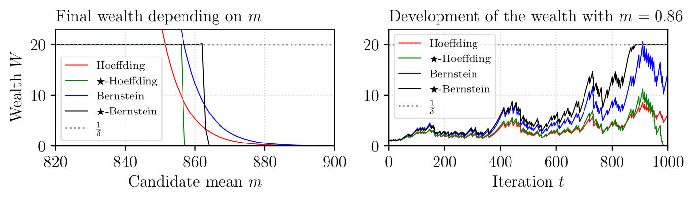
\[\ell_H^* = \sqrt{\frac{8\log\frac{1}{W_t\delta}}{n-t+1}}\]The effect is that when the algorithm has already accumulated substantial wealth, it can afford to be more conservative. Conversely, when it needs to make significant money in few remaining rounds, it will bet aggressively. This adaptive behavior is appropriate because the outcome of the betting game is fundamentally binary - we either accumulate $1/\delta$ wealth (rejecting the null) or we do not. We will demonstrate these observations in the upcomming figure. We further ntoe STaR-Hoeffding always produces shorter intervals than Hoeffding. The same can be observed for many other inequalities, such as the ones of Bernstein and Bennett, where we bound the cumulant generating function.
Limitations of Hoeffding Betting
One clear limitation is that Hoeffding betting does not adapt to $\sigma^2$, and thus not being able to provide the optimal width. This would be fixed by using Bernstein (or Bennett) betting which can be derived in the same spirit as above. However, there is still the problem that the betting game is very unfair in the small sample regime. Note that $\mathbb{E}[M(\ell)] \approx 1$ when $\ell \approx 0$, but as $\vert \ell\vert$ increases (i.e., when $n$ is small), the betting game will become more and more unfavorable, making it harder to reject the null hypotheses, and in turn making confidence intervals unnecessarily long. We need a better betting game that we now introduce.
The Main Algorithm: STaR-Bets
We consider the following fair betting game for refuting mean $m$: \(W_{i+1} = W_i(1- \ell(X_{i+1}-m)),\) where we require $\ell \leq 1/m$, then $W$ satisfies the supermartingale conditions. For our convenience, we consider the log-wealth which is for a constant bet:
\[\log W_n = \sum_{i=1}^n\log(1+\ell(X_i - m)) \approx \sum_{i=1}^n \ell(X_i - m) - \frac{\ell^2}{2}(X_i-m)^2\]by Taylor’s expansions. We are interested in achieving $\log W_n = \log\frac1\delta$, yielding
\[\ell^* = \sqrt\frac{2 \log \frac1\delta}{\sum_{i=1}^n (X_i-m)^2} \approx \sqrt\frac{2 \log \frac1\delta}{n \mathbb{E}[(X-m)^2]}.\]The quantity $\mathbb{E}[(X-m)^2]$ is unknown and we estimate it at time $t$ using $\frac1t \sum_{i=1}^t (X_i-m)^2 + n/t^2$ and thresholding at the maximal variance value $m(1-m)$ (recall that $X$ is supported on $[0,1]$). This estimator has the important property that it is consistent and that it is unlikely that it underestimates the underlying quantity. We have chosen this estimator for the convenience in proofs, but the sensitivity of the algorithm to the variance estimator is not high for reasonable estimators. Finally, we apply STaR technique on top, yielding bet at time $t$:
\[\ell^* = \sqrt\frac{2 \log \frac1{W_t\delta}}{(n-t+1) \min\left\{m(1-m), \left( n/t^2 + \frac1t \sum_{i=1}^t (X_i-m)^2 \right)\right\}}.\]Theoretical results
We show that the width of the resulting confidence interval is
\[\sigma\sqrt{\frac{(2+o(1))\log\frac{1}{\delta}}{n}}\]up to a $(1 + o(1))$ factor - matching the optimal rate! The $o$ considers scaling with $n$, the other factors are constant. We note that the actual result is a bit more subtle. Because the confidence interval is random, we cannot have such a deterministic statement, but we can have statement with arbitrarily high probability…
Experimental results
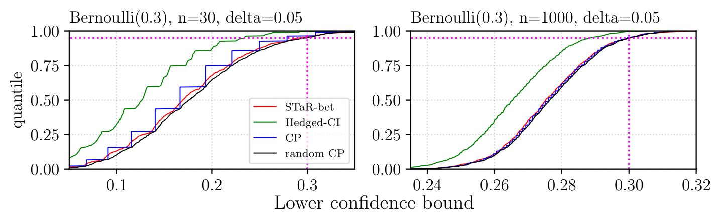
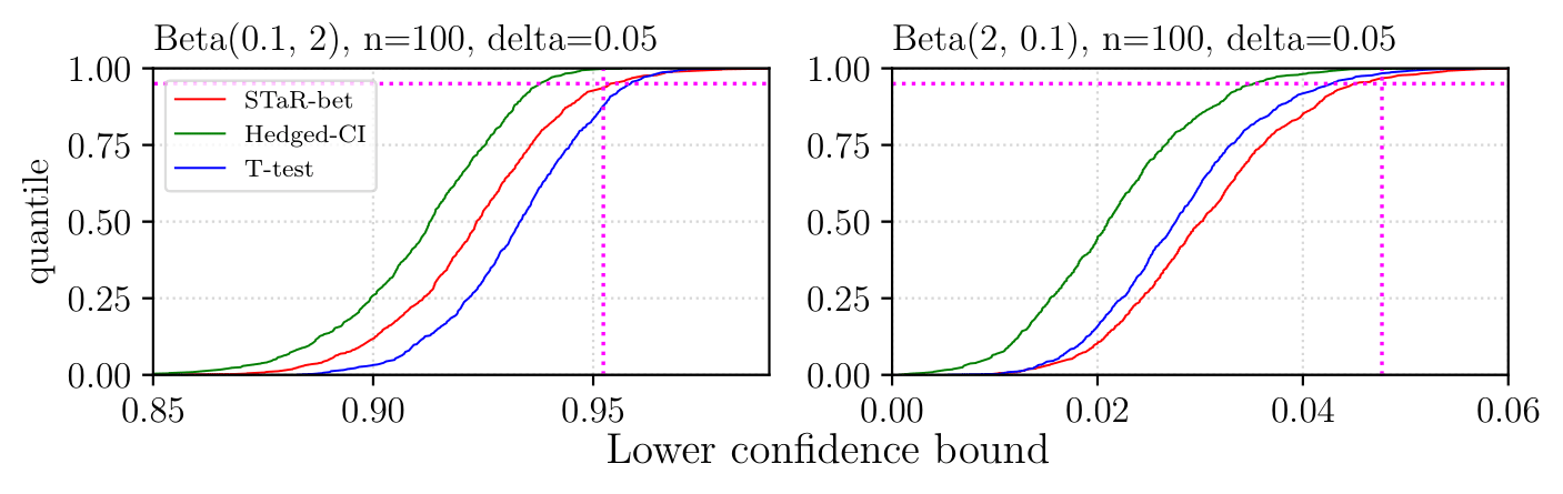
There is extensive experimental evidence in the paper. Here we only tease some Bernoulli results, where we demonstrate that STaR-Bets almost matches the optimal methods in Bernoulli estimation. We also provide some Beta distribution results, suggesting that STaR-bets outperforms (heuristical) T-test in the regimes where T-test actually have the desired coverage.
We use CDF figures: When a curve corresponding to a method passes through a point $(x,y)$, it means that the $y$-fraction (of $1000$ repetitions) of lower confidence bounds was smaller than $x$. The vertical magenta line shows the mean position, and the vertical one shows the $1-\delta$ quantile. We can see that in both cases, STaR-bet passes through the intersection, implying that the coverage is $\approx 1-\delta$.